Churn-Modeling
A predictive churn model is a powerful tool for identifying which of your customers will stop engaging with your business. With that information, you can built retention strategies, discount offers, email campaigns, and more that keep your high-value customers buying.
In [1]:
import numpy as np
import matplotlib.pyplot as plt
import pandas as pd
Importing the dataset
In [2]:
dataset = pd.read_csv('Churn_Modeling.csv')
X = dataset.iloc[:, 3:13].values
y = dataset.iloc[:, 13].values
In [3]:
dataset.head()
Out[3]:
In [4]:
print(X)
print('\n')
print(y)
Encoding categorical data (Geography, Gender)
In [5]:
from sklearn.preprocessing import LabelEncoder, OneHotEncoder
labelencoder_X_1 = LabelEncoder()
X[:, 1] = labelencoder_X_1.fit_transform(X[:, 1])
labelencoder_X_2 = LabelEncoder()
X[:, 2] = labelencoder_X_2.fit_transform(X[:, 2])
onehotencoder = OneHotEncoder(categorical_features = [1])
X = onehotencoder.fit_transform(X).toarray()
X = X[:, 1:]
In [6]:
print("X -> {}".format(X))
print('\n')
print("y -> {}".format(y))
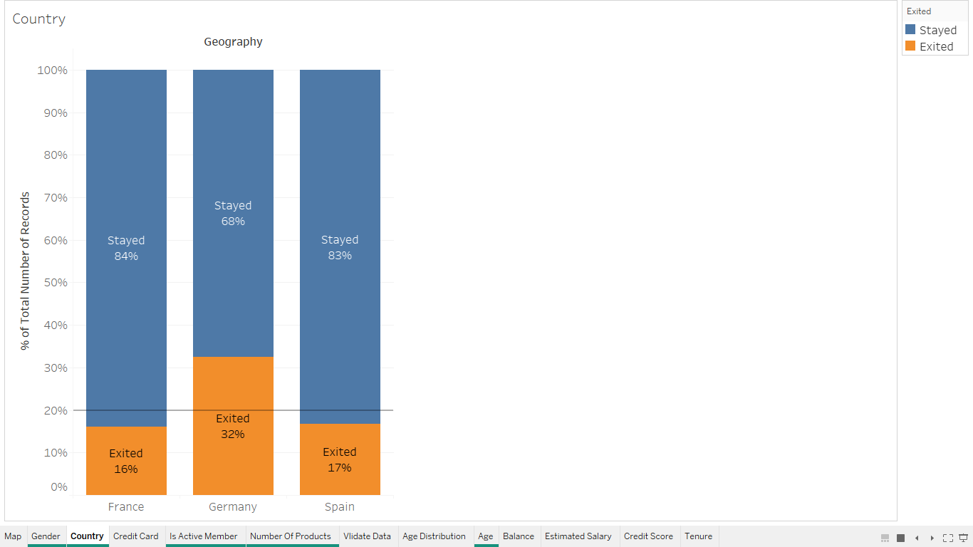
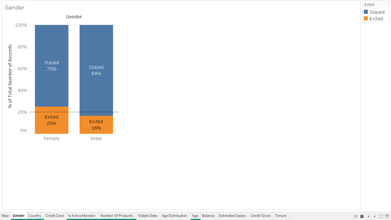
Exploratory Data Analysis
Statistical Description of the dataset
In [7]:
dataset.describe()
Out[7]:
In [8]:
dataset.columns
Out[8]:
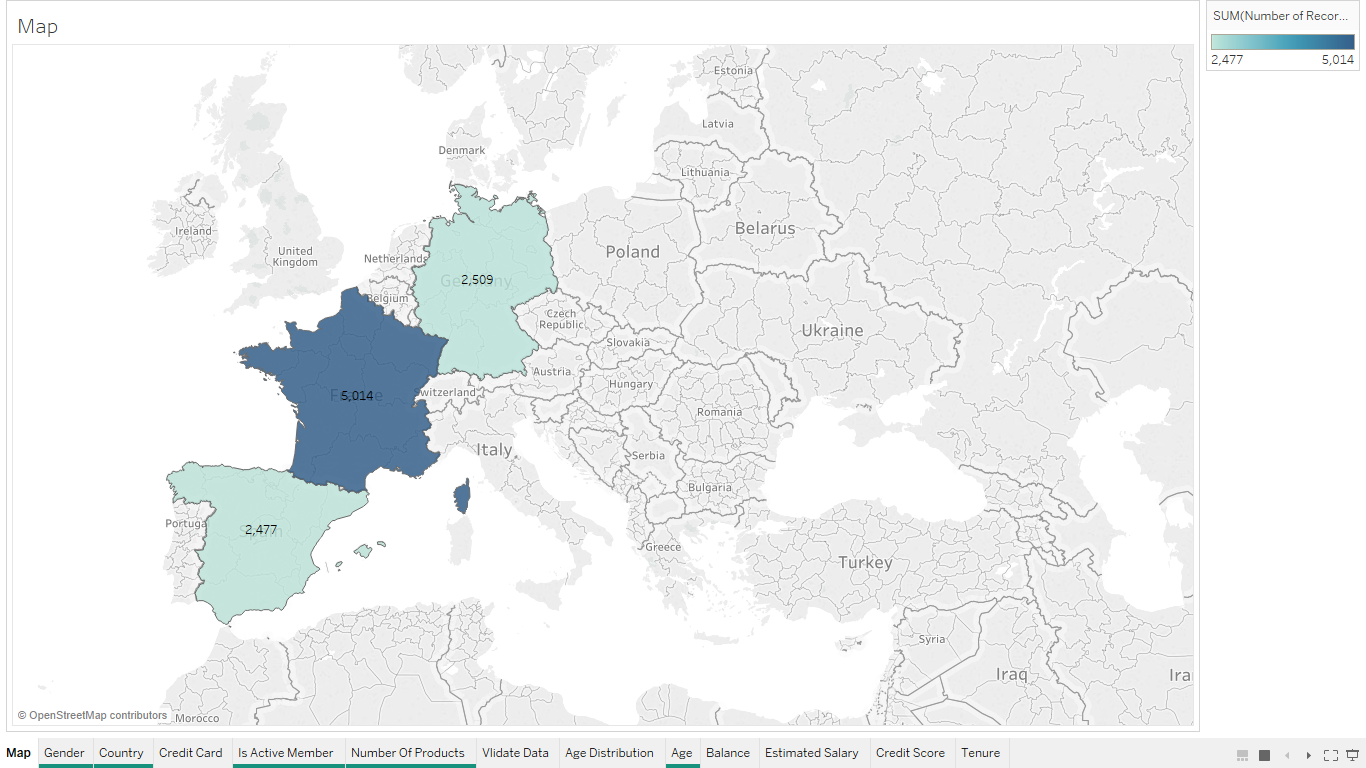
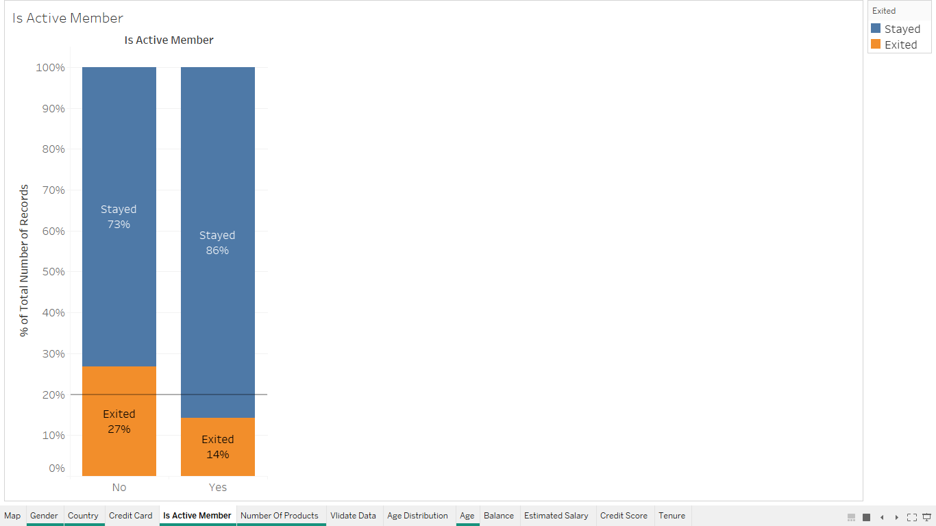
Based on Activity
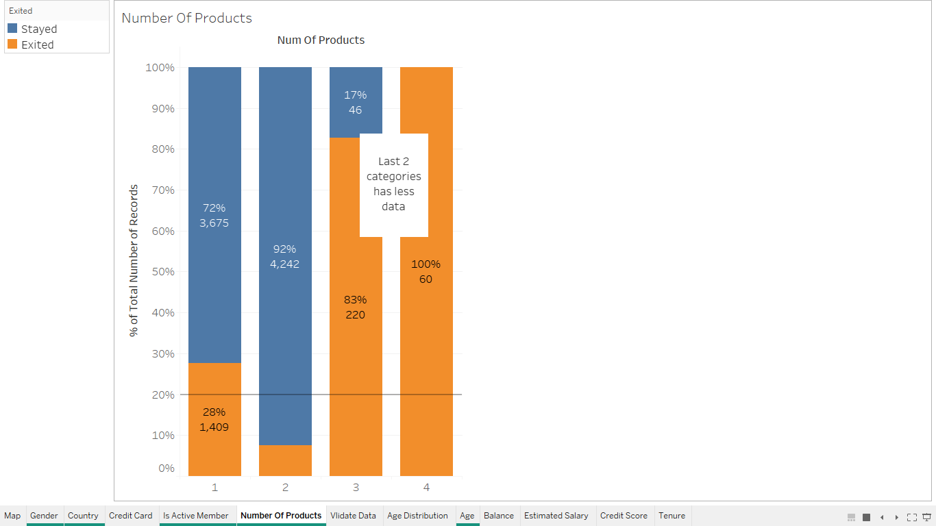
Based on number of products used
Splitting the dataset into the Training set and Test set
In [12]:
from sklearn.model_selection import train_test_split
X_train, X_test, y_train, y_test = train_test_split(X, y, test_size = 0.2, random_state = 0)
Feature Scaling
In [13]:
from sklearn.preprocessing import StandardScaler
sc = StandardScaler()
X_train = sc.fit_transform(X_train)
X_test = sc.transform(X_test)
In [14]:
print(X_train)
Applying various machine learning algorithms
Deploying Logistic Regression
In [15]:
from sklearn.linear_model import LogisticRegression
lr_classifier = LogisticRegression()
lr_classifier.fit(X_train, y_train)
y_lr_pred = lr_classifier.predict(X_test)
In [16]:
from sklearn.metrics import classification_report, confusion_matrix
print("confusion_matrix:\n {}".format(confusion_matrix(y_test, y_lr_pred)))
print("\nclassification_report: \n {}".format(classification_report(y_test, y_lr_pred)))
Deploying Support Vector Machine Classifier
In [17]:
from sklearn.svm import SVC
svm_classifier = SVC()
svm_classifier.fit(X_train, y_train)
y_svm_pred = svm_classifier.predict(X_test)
In [18]:
from sklearn.metrics import classification_report, confusion_matrix
print("confusion_matrix:\n {}".format(confusion_matrix(y_test, y_svm_pred)))
print("\nclassification_report: \n {}".format(classification_report(y_test, y_svm_pred)))
Deploying Random Forest Classifier
In [19]:
from sklearn.ensemble import RandomForestClassifier
Rf_classifier = RandomForestClassifier()
Rf_classifier.fit(X_train, y_train)
y_rf_pred = Rf_classifier.predict(X_test)
In [20]:
from sklearn.metrics import classification_report, confusion_matrix
print("confusion_matrix:\n {}".format(confusion_matrix(y_test, y_rf_pred)))
print("\nclassification_report: \n {}".format(classification_report(y_test, y_rf_pred)))
Building an Artificial Neural Network
In [21]:
# Importing the Keras libraries and packages
import keras
from keras.models import Sequential
from keras.layers import Dense
In [22]:
# Initialising the ANN
classifier = Sequential()
In [23]:
# Adding the input layer and the first hidden layer
classifier.add(Dense(units = 6, kernel_initializer = 'uniform', activation = 'relu', input_dim = 11))

# Adding the second hidden layer
classifier.add(Dense(units = 6, kernel_initializer = 'uniform', activation = 'relu'))

# Adding the output layer
classifier.add(Dense(units = 1, kernel_initializer = 'uniform', activation = 'sigmoid'))
Training the ANN
In [24]:
# Compiling the ANN
classifier.compile(optimizer = 'adam', loss = 'binary_crossentropy', metrics = ['accuracy'])
In [25]:
# Fitting the ANN to the Training set
classifier.fit(X_train, y_train, batch_size = 10, epochs = 100)
Out[25]:
In [26]:
# Predicting the Test set results
y_pred = classifier.predict(X_test)
y_pred = (y_pred > 0.5)
In [27]:
# Making the Confusion Matrix
from sklearn.metrics import confusion_matrix
cm = confusion_matrix(y_test, y_pred)
In [28]:
print (cm)
In [29]:
from sklearn.metrics import classification_report
print(classification_report(y_test, y_pred))
In [30]:
from sklearn.decomposition import PCA
pca = PCA(n_components=2)
X_pca = pca.fit_transform(X_train)
In [31]:
X_pca
Out[31]:
In [32]:
pca_df = pd.DataFrame(data=X_pca, columns=["pca 1", "pca 2"])
pca_df["pred"] = y_train
Evaluation
Here there's a close competition but Support Vector Machines win with the Precision = 0.86, Recall =0.86 and F1-score = 0.85.